
FROGS Core
Galaxy
- Get Started ▾
- Reads processing
- Remove chimera
- Cluster/ASV filters
- Taxonomic affiliation
- Phylogenetic tree building
- ITSx
- Read demultiplexing
- Affiliatio filters
- Affiliation postprocessing
- Abundance normalisation
- Convert Biom file to TSV file
- Convert TSV file to Biom file
- Cluster/ASV report
- Affiliation report
Main tools
Optional tools
CLI
- Get Started
- Reads processing
- Remove chimera
- Cluster/ASV filters
- Taxonomic affiliation
- Phylogenetic tree building
- ITSx
- Read demultiplexing
- Affiliation filters
- Affiliation postprocessing
- Abundance normalisation
- Convert Biom file to TSV file
- Convert TSV file to Biom file
- Cluster/ASV report
- Affiliation report
Main tools
Optional tools
Reads processing
Context
Denoising refers to the process of correcting sequencing errors that occur during high-throughput sequencing of amplicons.
These errors can originate from PCR amplification or from the sequencing platform itself (e.g., Illumina, long-read technologies,
or older 454 systems). They typically appear as spurious singletons or low-abundance variants that differ by only one or a few
bases from the actual biological sequences. Tools such as denoising.py in FROGS implement strategies such as clustering (e.g.,
with Swarm) or statistical inference (e.g., with DADA2) to distinguish real variants (ASVs) from sequencing noise.
How it does
This tool cleans raw sequencing data before denoising.
To achieve this, it relies on well-established preprocessing tools:
Then the tool can clustered sequences using either:
- Swarm, which groups sequences based on local connectivity and a user-defined distance (e.g., 1 nucleotide difference), producing robust clusters without relying on arbitrary global thresholds.
- DADA2, which applies a statistical error model to distinguish true biological sequences from sequencing errors, allowing inference of exact sequence variants with very high resolution.
Together, these steps ensure that downstream analyses are based on accurate, high-quality ASVs, reducing the impact of technical artifacts such as primer sequences, incomplete overlaps, or sequencing errors. It is possible to perform cleanup only with the
To achieve this, it relies on well-established preprocessing tools:
- Cutadapt is used to detect and remove sequencing primers or adapters from the reads.
- Delete sequences without good primers. In the context of amplicon data, primers must be trimmed because they can interfere with downstream clustering/denoising and taxonomic assignment.
Cutadapt also allows mismatches, making it robust for real-world data where primer binding is not always perfect.
- Merging of R1 and R2 reads with vsearch, flash or pear (only in command line) into single continuous sequences when their overlaps are sufficient.
- Delete sequence with not expected lengths
- Delete sequences with ambiguous bases (N)
- Dereplication
- + removing homopolymers (size = 8 ) for 454 data
- + quality filter for 454 data
Then the tool can clustered sequences using either:
- Swarm, which groups sequences based on local connectivity and a user-defined distance (e.g., 1 nucleotide difference), producing robust clusters without relying on arbitrary global thresholds.
- DADA2, which applies a statistical error model to distinguish true biological sequences from sequencing errors, allowing inference of exact sequence variants with very high resolution.
Together, these steps ensure that downstream analyses are based on accurate, high-quality ASVs, reducing the impact of technical artifacts such as primer sequences, incomplete overlaps, or sequencing errors. It is possible to perform cleanup only with the
--process preprocess-only option of denoising. N.B. : Long reads
DADA2 needs to see the same sequences multiple times to model sequencing errors. If almost all sequences are unique (as is often the case with very long PacBio reads), DADA2 cannot function properly because it does not have enough information to distinguish true errors from true biological variations.
If the duplication rate is less than 10% (i.e., if the number of unique sequences > 0.9 × the total number of reads), then DADA2 is not appropriate.
The knowledge of your data is essential. You have to answer the following questions to choose the parameters:
If the duplication rate is less than 10% (i.e., if the number of unique sequences > 0.9 × the total number of reads), then DADA2 is not appropriate.
The knowledge of your data is essential. You have to answer the following questions to choose the parameters:
- Sequencing technology?
- Targeted region and the expected amplicon length?
- Have reads already been merged?
- Have primers already been deleted?
- What are the primers sequences?
Configuration: Short reads (16S V3V4 use cases)
Here are the answers for this dataset:
First, select the

The dataset has R1 and R2 files for one sample. Select
The input file is an archive. For your own data, it will be important to know how create an archive.
Select your file after uploading your data . It can be automatically detected.

R1 and R2 are both
We choose to allow only a 0.1 mismatch rate in the overlap region between R1 and R2 reads.

You can choose either

We know that our amplicons are approximately 450 bp long. After trying different minimum and maximum values, we settled on a minimum amplicon length of

We have the primers that were used, so we select


Don't forget to click on the button :
- Sequencing technology
- Illumina
- 454
- long reads
- Type of data
- R1 and R2 files for one sample
- One file by sample (R1 and R2 already merged or single-end technology data)
- Amplicon expected length
- Reads are mergeable: V3-V4 region is ~450-bp. So reads should overlap
- Reads are not mergeable
- Reads are are both mergeable and unmergeable
- Primers sequences
- Primers are still present: V3F(5’-ACGGRAGGCWGCAGT-3’) and V4R (5’-TACCAGGGTATCTAATCCT-3’) have been used for the first amplification
- Primers have already been removed
- Reads size
- 250 bp as seen previously
First, select the
Main 1.a. Denoising of short reads tool.
The dataset has R1 and R2 files for one sample. Select
Paired-end reads. The input file is an archive. For your own data, it will be important to know how create an archive.
Select your file after uploading your data . It can be automatically detected.
R1 and R2 are both
250 bp.We choose to allow only a 0.1 mismatch rate in the overlap region between R1 and R2 reads.
You can choose either
Flash or Vsearch as the read merging tool. In our case, we want to use Vsearch and discard any unmerged reads.
We know that our amplicons are approximately 450 bp long. After trying different minimum and maximum values, we settled on a minimum amplicon length of
420 bp and a maximum length of 470 bp.
We have the primers that were used, so we select
Yes and enter them. Make sure you put the primers in the correct orientation. You can use this tool to obtain the reverse complement.
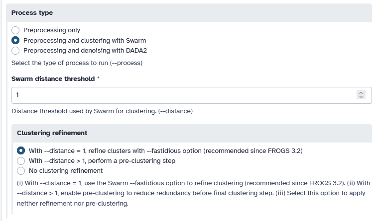
Swarm
We will show you an example of the output fromSwarm clustering with a distance of 1 between neighbouring sequences. We are using the fastidious option.
or DADA2
But also an example withDADA2 by choosing the Pseudo pooling, samples will be pseudo-pooled prior to sample inference method.
Don't forget to click on the button :
Interpretation: Short reads (16S V3V4 use cases)
Swarm Results
Let look at the HTML file to see the result of denoising.You have three panels: Denoising, Cluster distribution, and Sample distribution. Here, we will focus primarily on the Denoising panel.

Since the Cluster distribution and Sample distribution panels are common to multiple tools, a more detailed interpretation with vizualisation of these panels can be found in the Cluster Stat section .

This bar plot shows the number of sequences that do not pass the filters. At the end of the filtering process, we have 1,156,905 sequences.
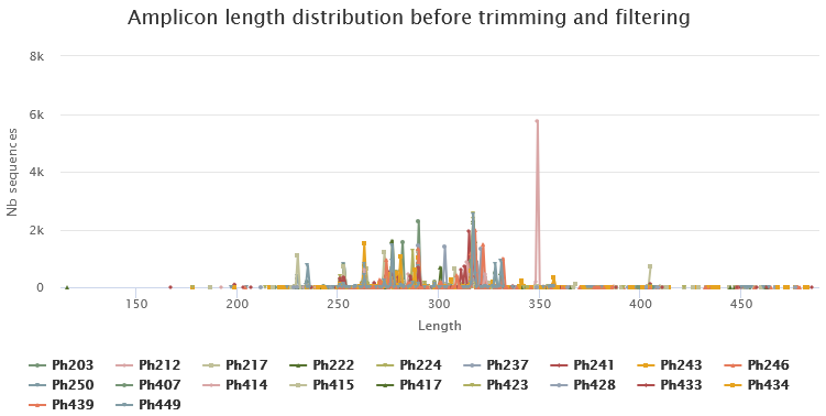
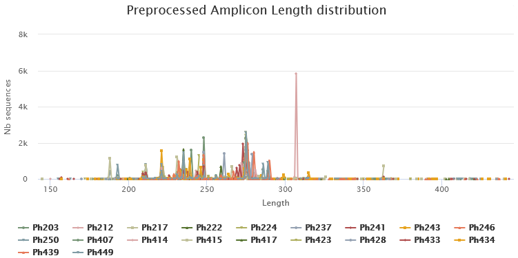
Below you will find a table showing details on merged sequences. Display all sequences (1) and select all samples (2). You can then click on Display amplicon lengths (3) and Display preprocessed amplicon lengths (4).


We observe that the majority of sequences are ~425 nt long.
The other tabs give information about clusters. They show classical characteristics of clusters built with swarm:
- A lot of clusters: 142,515
- ~81.63% of them are composed of only 1 sequence
DADA2 Results
Let look at the HTML file to check what happened.- 87.39% of raw reads are kept (1,200,783 sequences from 1,374,011)
- 8,580 Clusters, ~23.24% of them composed of only 1 sequences

Configuration: Short reads (ITS use cases)
Here are the answers for this dataset:
First, select the
The dataset has R1 and R2 files for one sample. Select
Select your file after uploading your data. It can be automatically detected.
Paste/Fetch data :

R1 and R2 are both
We choose to allow only a 0.1 mismatch rate in the overlap region between R1 and R2 reads.
You can choose either

We know that our amplicons are approximately 450 bp long. After trying different minimum and maximum values, we settled on a minimum amplicon length of

We have the primers that were used, so we select

Don't forget to click on the button :
- Sequencing technology
- Illumina
- 454
- long reads
- Type of data
- R1 and R2 files for one sample
- One file by sample (R1 and R2 already merged or single-end technology data)
- Amplicon expected length
- Reads are mergeable.
- Reads are not mergeable
- Reads are are both mergeable and unmergeable, unmerged reads will be artificially combined with 100 N to allow further processing.
- Primers sequences
- Primers are still present: V3F(5’-CTTGGTCATTTAGAGGAAGTAA-3’) and V4R (5’-GCATCGATGAAGAACGCAGC-3’) have been used for the first amplification
- Primers have already been removed
- Reads size
- 250 bp
First, select the
Main 1.a. Denoising of short reads tool.
The dataset has R1 and R2 files for one sample. Select
Paired-end reads. Select your file after uploading your data. It can be automatically detected.
Paste/Fetch data :
- https://web-genobioinfo.toulouse.inrae.fr/~formation/15_FROGS/current/ITS_fast.tar.gz
- https://web-genobioinfo.toulouse.inrae.fr/~formation/15_FROGS/current/ITS_fast_replicates.tsv
R1 and R2 are both
250 bp.We choose to allow only a 0.1 mismatch rate in the overlap region between R1 and R2 reads.
You can choose either
Flash or Vsearch as the read merging tool. In our case, we want to use Vsearch and and click on Yes to retain the unmerged reads that will be artificially combined with 100N for further processing.
We know that our amplicons are approximately 450 bp long. After trying different minimum and maximum values, we settled on a minimum amplicon length of
420 bp and a maximum length of 470 bp.
We have the primers that were used, so we select
Yes and enter them. Make sure you put the primers in the correct orientation. You can use this tool to obtain the reverse complement.
Swarm
We will show you an example of the output fromSwarm clustering with a distance of 1 between neighbouring sequences. We are using the fastidious option.
Don't forget to click on the button :
Interpretation: Short reads (ITS use cases)
Swarm Results
Let look at the HTML file to see the result of denoising.You have three panels: Denoising, Cluster distribution, and Sample distribution. Here, we will focus primarily on the Denoising panel.
Since the Cluster distribution and Sample distribution panels are common to multiple tools, a more detailed interpretation with vizualisation of these panels can be found in the Cluster Stat section .

This bar plot shows the number of sequences that do not pass the filters. At the end of the filtering process, we have 198,191 sequences. We also see the number of artificially recombined reads, 47,594 reads.
Below you will find a table showing details on merged sequences. Display all sequences (1) and select all samples (2). You can then click on Display amplicon lengths (3) and Display preprocessed amplicon lengths (4).

ITS sequence sizes vary greatly.
Details on artificial combined sequences

This table provides information on artificial combined sequences by sample.
The other tabs give information about clusters. They show classical characteristics of clusters built with swarm:
- A lot of clusters: 50,883
- 97.9% of them are composed of only 1 sequence